Preface

Linear algebra can pop up in unexpected places. When I was prepping for internship interviews last year, I stumbled upon a beautiful way to compute Fibonacci numbers. I coded up a few other methods for comparison, starting with naive recursion.

The differences were hilarious. The linear-algebra approach blows every other method out of the park!

Yup, I’m talking about the brown curve. The curves show the time it took to compute the N-th Fibonacci number. Lower is better.

Let’s look at the methods one-by-one. We’ll start with the simplest and work our way up.

Let’s go!

Method 1: Recursion

The simplest method implements the recursive nature of Fibonacci numbers: \(F(n) = F(n-1) + F(n-2)\), with \(F(0) = 0\) and \(F(1) = 1\). This is most people’s first programming exercise involving recursion.

def fibonacci_recursion(k):
    if k==1:
        return 1
    elif k==0:
        return 0
    else:
        return fibonacci_recursion(k-1) + fibonacci_recursion(k-2)

The x-axis denotes integers and y-axis denotes the time it took for a particular method to compute the N-th fibonacci number. The time per integer is averaged over 500 independent runs of the experiment.

Looks like exponential computation complexity, eh?

Note that both fibonacci_recursion(n) and fibonacci_recursion(n-1) require \(F(n-2)\), but both compute it independently.

Let’s visualize the recursion tree for \(F(8)\).

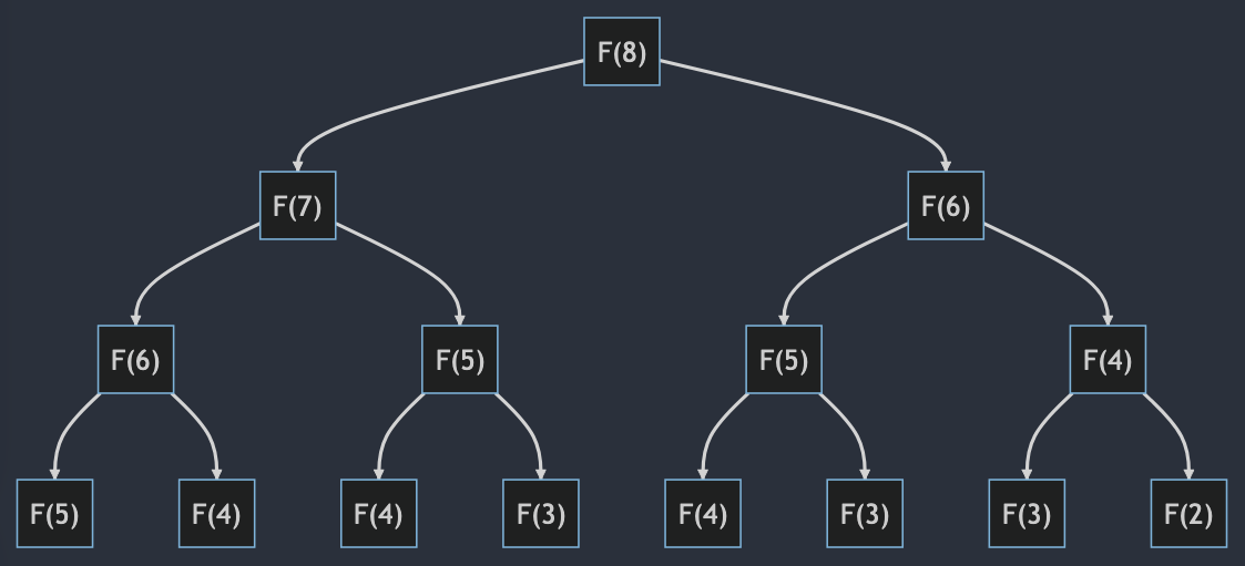Depiction of the \(O(2^n)\) computations for computing \(F(n)\)

The tree grows by a factor of \(2\) at each level—exponential complexity. There is so much repeated computation!

Method 2: Recursion with bookkeeping

An obvious optimization is to store every \(F(k)\) that is computed.

def fibonacci_recursion_with_bookkeeping(k):

    # create a list to store all the computed numbers
    fib_list = np.zeros(k + 1) - 1
    # fib_list[n] = -1 indicates the n-th Fibonacci number hasn't been computed
    fib_list[0] = 0
    fib_list[1] = 1

    # the recursive function
    def _fibonacci_recursion_with_bookkeeping(k):
        # don't compute the number again if we've computed it once
        if fib_list[k] != -1:
            return fib_list[k]
        else:
            fib_list[k] = _fibonacci_recursion_with_bookkeeping(k-1) + _fibonacci_recursion_with_bookkeeping(k-2)
            return fib_list[k]

    return _fibonacci_recursion_with_bookkeeping(k)

Bookkeeping certainly helps. It cuts down on lots of redundant computation.

Method 2 only requires \(O(n)\) computation, but the recursive function is called \(O(2^n)\) times.

We can do even better by getting rid of the recursion altogether while storing all the results we’ve computed so far.

Method 3: Dynamic Programming

def fibonacci_dynamic_programming(k):

    fib_list = np.zeros(k + 1, dtype=object)
    fib_list[1] = 1

    for i in range(2, k+1):
        fib_list[i] = fib_list[i-1] + fib_list[i-2]

    return fib_list[k]

Pretty good already.

Now let’s see how linear algebra comes in.

Buckle up, we are going to get technical!

Method 4: Matrix power

Let us look at the Fibonacci formula again: \(\begin{aligned} F(k+1) &= F(k) + F(k-1). \end{aligned}\) Consider the vector: \(\begin{aligned} x_{k} = \begin{bmatrix} F(k) \\ F(k-1) \\ \end{bmatrix}. \end{aligned}\)

Then \(F(k+1) = [1, 1]^\top x_k\). Similarly, \(F(k) = [1, 0]^\top x_k\). Combining the two, \(\begin{aligned} F(k+1) &= [1, 1]^\top x_k, \\ F(k) &= [1, 0]^\top x_k, \\ \implies \begin{bmatrix} F(k+1) \\ F(k) \\ \end{bmatrix} &= \begin{bmatrix} 1 & 1 \\ 1 & 0 \\ \end{bmatrix} x_k. \\ \text{or}\quad x_{k+1} &= \begin{bmatrix} 1 & 1 \\ 1 & 0 \\ \end{bmatrix} x_k. \end{aligned}\)

Let’s call this matrix \(A = \begin{bmatrix} 1 & 1 \\ 1 & 0 \\ \end{bmatrix}\). Then,

\(F(k)\) is the second element of \(x_{k+1}\), that is, \(F(k) = x_{k+1}[1] = (A^{k} x_1)[1]\).

So using linear algebra, we can calculate \(F(k)\) by simply computing the second element of \(A^{k} x_1\).

def fibonacci_linalg_powers(k):
    A = np.array([[1, 1],
                  [1, 0]], dtype=int)
    x_1 = np.array([1, 0])

    A_power = A
    for i in range(2, k+1):
        A_power = A @ A_power   # '@' denotes matrix multiplication

    return (A_power@x_1)[1]

The naive matrix-power method is faster than the recursion-based methods, but much slower than dynamic programming.

To compute \(F(n)\), this method involves \(n\) matrix multiplications. That is, this is also an \(O(n)\) method.

But why compute the powers one by one?

Method 5: Matrix power by iterative squaring

To compute \(A^8\) starting from \(A\),

• multiply \(AA\) to get \(A^2\),
• multiply \(A^2 A^2\) to get \(A^4\),
• multiply \(A^4 A^4\) to get \(A^8\).

Just three operations. More precisely, \(\log_2(8)\) operations. Nice!

But what about numbers that are not powers of \(2\)?

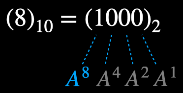
Binary representation to the rescue!

Recall: \((8)_{10} = (100)_{2}\). Starting from \(\bf{A}\), we kept squaring the powers till we reached the 1 in the binary representation of 8.

Now consider 11:

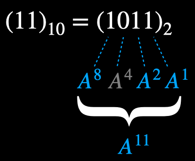
If we multiple the powers corresponding to the 1s in the binary representation of 11, we get \(\bf{A}^{11}\).

That’s neat, because we will be computing all of those powers en-route to computing the largest power. So we can just multiply them all the powers to get the right result!

def fibonacci_linalg_powers_better(k):
    A = np.array([[1, 1],
                  [1, 0]], dtype=int)
    x = np.array([1, 0])

    A_power = A
    result = np.eye(2, dtype=int)
    while k > 0:
        if k % 2:
            result = result @ A_power
            k -= 1
        k = k // 2
        A_power = A_power @ A_power

    return (result@x)[1]

Method 5 of computing matrix powers by iterative squaring is slower than DP for smaller numbers, but the speedup is apparent for larger numbers.

As you likely have guessed, this is an \(O(\log n)\) method.

Guess what the spiky-but-regular pattern is?

Hint: note which numbers correspond to a dip in computation time.

Method 6: Diagonalization

We’re computing matrix powers. Can we leverage the diagonalization property?

If \(\mathbf{A}\) can be diagonalized, instead of computing costly matrix powers, we can just cheaply compute the powers of scalars!

This is clearly desirable. So let’s do it.

Recall \(\mathbf{S}\) is composed of the eigenvectors of \(\mathbf{A}\) arranged row-wise and \(\Lambda\) is a diagonal matrix with the corresponding eigenvalues along the diagonal. So we need to compute the eigenvalues and eigenvectors of \(\mathbf{A}\).

First, the eigenvalues:

For these eigenvalues, we obtain the eigenvectors: \(\mathbf{x}_1 = [\lambda_1, 1]^\top, \mathbf{x}_2 = [\lambda_2, 1]^\top\).

Thus, \(\begin{aligned} \mathbf{S} = \begin{bmatrix} \lambda_1 & \lambda_2 \\ 1 & 1 \end{bmatrix}, \quad \Lambda = \begin{bmatrix} \lambda_1 & 0 \\ 0 & \lambda_2 \end{bmatrix}. \end{aligned}\)

And \(\mathbf{S}^{-1} = \frac{1}{\lambda_1 - \lambda_2} \begin{bmatrix} 1 & -\lambda_2 \\ -1 & \lambda_1 \end{bmatrix}\).

So, \(\begin{aligned} \mathbf{A} = \mathbf{S} \Lambda \mathbf{S}^{-1} = \frac{1}{\lambda_1 - \lambda_2} \begin{bmatrix} \lambda_1 & \lambda_2 \\ 1 & 1 \end{bmatrix} \begin{bmatrix} \lambda_1 & 0 \\ 0 & \lambda_2 \end{bmatrix} \begin{bmatrix} 1 & -\lambda_2 \\ -1 & \lambda_1 \end{bmatrix} \end{aligned}\)

Now,

Then,

The \(k\)-th Fibonacci number is the nearest integer of \((\mathbf{A} \mathbf{x}_1)[1]\):

That’s it!

The concept of diagonalization has enabled the computation of Fibonacci numbers by simply using powers of scalar numbers!

def fibonacci_linalg_diagonalization(k):
    lambda1 = (1 + np.sqrt(5)) / 2
    lambda2 = (1 - np.sqrt(5)) / 2

    return round((lambda1**k - lambda2**k)/(lambda1 - lambda2))

Lol

That’s an incredible speedup!

As one would suspect, it’s much cheaper to compute the powers of scalars than of matrices.

Still, doesn’t it seem ludicrous that the line is flat? Surely computing a larger power should take more time than computing a smaller one.

Maybe the constant ahead of \(O(n)\) is small and doesn’t really show up for 120 Fibonacci numbers we are computing.

So here’s the graph for the first 1000 Fibonacci numbers:

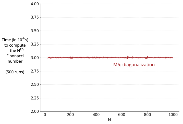Yup…!

Note: This line is flatter than the one we saw earlier despite having a smaller y-axis scale. That’s because I finally removed outliers (using Tukey’s method with k=1.5) because at the time scales we are operating in (microseconds), noise can really screw up the results.

Isn’t it incredible?

That led me to the rabbit-hole of fast exponentiation. But that’s another blog post :)

Till I write this new post, you can google ‘shortest addition chains’.

Wrapping up

I enjoyed this journey. I hope you did too :)

Knowledge is power. Connections between seemingly unrelated topics can unlock ideas that are greater than the sum of its parts!

Stay curious :)

For feedback or discussion, email/Slack or DM me however.

_{Notes:
1: I ran the above experiments on a 2021 M1 Pro. The exact numbers may differ on other machines but the trends should remain the same.
2: I’ve used the native object dtype everywhere because it does not overflow (at the cost of an increased memory footprint). You can learn more about it here and here.
3: Thanks to Roshan for pointing out that the simple diagonalization code above starts having rounding errors for larger Fibonacci numbers (since \(\sqrt{5}\) is an irrational number). I found this neat Decimal package that resolves this issue (at the cost of a small constant time addition).
4: We can make the diagonalization method even faster by (a) simplifying the denominator to \(\sqrt{5}\), and (b) ignoring \(\lambda_2^k\) as it will be almost zero for most \(k\).
5: Thank you Shivam for proof-reading!
6: Thank you Gilbert Strang for writing a wonderful textbook on Linear Algebra :)}