
Preface
We have all seen videos of like the following, of planets revolving around a star:
 |
|---|
| Figure 1: Three bodies revolving around a central body with different angular velocities |
Simple orbital mechanics tells us that the angular velocity of an orbiting body is inversely proportional to its distance from the central body.
Turns out, under specific conditions, the latter can also be true!
 |
|---|
| Figure 2: Three bodies revolving around a central body with the same angular velocity |
For every orbiting body, there exist four points in its vicinity where a tiny body can have the same angular velocity as the primary body around a central celestial body. This post outlines my journey of understanding these Lagrange points—and hopefully yours as well.
 |
|---|
| Figure 3: Two small bodies at the L1 and L2 points of a two-body system consisting of a planet revolving around a star. |
Background
First, let’s quickly review some orbital mechanics.
Define:
- \(m_s\): mass of the Sun
- \(m_e\): mass of Earth
- \(G\): the Gravitational constant
- \(R\): average distance between the Sun and Earth. For simplicity, we assume that Earth’s orbit around the Sun is circular.
Earth is in a stable orbit around the Sun, which means the gravitational force exerted by the Sun on Earth is balanced by the centripetal force experienced by Earth due to its revolution around the Sun. That is,
\[\frac{G m_s m_e}{R_e^2} = m_e\, \omega_e^2 R_e.\]This implies: \(\omega_e = \sqrt{\frac{Gm_s}{R_e^3}}\). This equation clearly shows that objects further away from the Sun have a lower angular velocity (as seen in Figure 1).
Now, the gravitational force of the Sun on a satellite orbiting the Sun at a distance \(r\) from Earth (between Earth and the Sun) is \(F_s = \frac{G m_s m_{sat}}{(R_e-r)^2}\) and that of Earth on the satellite is \(F_e = \frac{G m_e m_{sat}}{r^2}\). The centripetal force experienced by the satellite due to its revolution around the Sun is \(F_{cent} = m_{sat} \omega^2 (R_e-r)\).
Deriving the L1 point
Satellites at Lagrange points rotate around the sun at the same angular velocity as that of the smaller body—in this case, Earth. So, at L1, \(\omega=\omega_e\) and \(F_s = F_e + F_{cent}\). Solving for \(r\),
\[\begin{align*} \frac{G m_s m_{sat}}{(R-r)^2} &= \frac{G m_e m_{sat}}{r^2} + m_{sat} \omega^2 (R-r) \\ \implies \frac{G m_s}{(R-r)^2} &= \frac{G m_e}{r^2} + \omega^2 (R-r). \end{align*}\]Substituting the value of \(\omega\),
\[\begin{align*} \frac{G m_s}{(R-r)^2} &= \frac{G m_e }{r^2} + \frac{Gm_s}{R^3} (R-r) \\ \implies \frac{m_s}{(R-r)^2} &= \frac{m_e }{r^2} + \frac{m_s}{R^3} (R-r). \end{align*}\]This is a fifth-degree polynomial in \(r\).
I tried finding its solutions using pen and paper but all I ended up doing was wasting using a lot of ink.
Wolfram Alpha didn’t help either; I couldn’t make any sense of its output.
At this point, I went to Wikipedia to look up the ‘answer’. It had an approximate answer, quoting the quintic equation had no closed-form solution. That explained my struggles.
Even if a closed-form solution doesn’t exist, we should still be able to approximate it.
My first attempt was through visualizing all the forces to get an idea of where they cancel out.
Force visualization
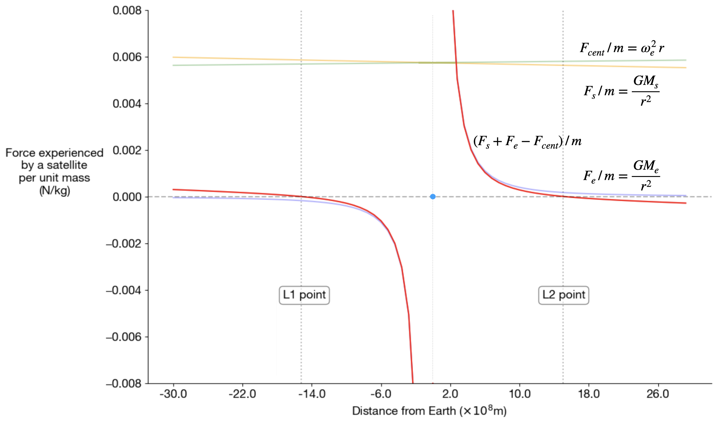
The three forces acting on the satellite are the two gravitational forces due to the attraction by the Sun and Earth—\(F_s\) and \(F_e\) respectively—as well as the centripetal force due to the revolution around Sun—\(F_{cent}\). For simplicity, we will plot the forces per unit mass of the satellite.
 |
|---|
| Figure 4: Forces acting on a satellite per unit mass. The distance \(r\) is measured from the sun but the x-ticks are shown w.r.t. Earth for better interpretability. |
There is a lot going on in the plot, so let us consider a few basic things one at a time:
- The centripetal force for a fixed angular velocity (\(\omega_e\), that of Earth around the Sun) increases with distance from the Sun. At the scale of the plot, this is indicated by a small positive slope (green).
- At the scale of the plot, the gravitational force due to the Sun appears almost constant, but with a perceptible negative slope (orange).
- The gravitational force due to Earth is symmetric (blue), with the direction towards the sun indicated with a negative sign.
The red line indicates the sum of forces experienced by a satellite per unit mass. It is zero at roughly \(1.5 * 10^9\)km on either side of Earth—our first (visual) estimate of the L1 and L2 points.
The estimate is quite rough, but it can be made more precise with just a few additions to the code I wrote to generate the plot.
Numerical estimation
This piece of code incrementally estimates the distance where the forces balance out by starting close to Earth and gradually increasing the distance towards the Sun. The code should converge to the L1 point after enough iterations.
import math

G  = 6.67e-11                     # the Gravitational constant (m^3/(kg s^2))
m1 = 1.989e30                     # mass of Sun (kg)
m2 = 5.9722e24                    # mass of Earth (kg)
R  = 1.52e11                      # average distance between Sun and Earth (m)

w_m2 = math.sqrt(G * m1 / R**3)   # angular velocity of Earth around Sun (rad/s)

F1_by_m = lambda l1: G * m1 / (R - l1)**2    # gravitational force per unit mass due to Sun (m/s^2)
F2_by_m = lambda l1: G * m2 / (l1)**2        # gravitational force per unit mass due to Earth (m/s^2)
F_cent_by_m = lambda l1: w_m2**2 * (R - l1)  # centrifugal force per unit mass when orbiting around Sun with Earth's angular velocity (m/s^2)

l1 = 1e4                # lower bound of the guess, starting at some small value close to Earth (m)
delta = 1e8             # how much to increment each guess (m)
upper_bound = R/2       # upper bound of the guess, starting at a large value far from Earth (m)

num_increments = 0
for i in range(20):
    print(f'Iteration {i}: start={l1}, end={upper_bound}, delta={delta}')
    while l1 < upper_bound:
        if F2_by_m(l1) + F_cent_by_m(l1) < F1_by_m(l1):
            break
        else:
            l1 += delta
    upper_bound = l1
    l1 -= delta
    delta /= 2
    Iteration 0: start=10000.0, end=76000000000.0, delta=100000000.0
    Iteration 1: start=1500010000.0, end=1600010000.0, delta=50000000.0
    Iteration 2: start=1500010000.0, end=1550010000.0, delta=25000000.0
    Iteration 3: start=1500010000.0, end=1525010000.0, delta=12500000.0
    Iteration 4: start=1512510000.0, end=1525010000.0, delta=6250000.0
    Iteration 5: start=1512510000.0, end=1518760000.0, delta=3125000.0
    Iteration 6: start=1512510000.0, end=1515635000.0, delta=1562500.0
    Iteration 7: start=1514072500.0, end=1515635000.0, delta=781250.0
    Iteration 8: start=1514853750.0, end=1515635000.0, delta=390625.0
    Iteration 9: start=1515244375.0, end=1515635000.0, delta=195312.5
    Iteration 10: start=1515244375.0, end=1515439687.5, delta=97656.25
    Iteration 11: start=1515342031.25, end=1515439687.5, delta=48828.125
    Iteration 12: start=1515342031.25, end=1515390859.375, delta=24414.0625
    Iteration 13: start=1515342031.25, end=1515366445.3125, delta=12207.03125
    Iteration 14: start=1515354238.28125, end=1515366445.3125, delta=6103.515625
    Iteration 15: start=1515354238.28125, end=1515360341.796875, delta=3051.7578125
    Iteration 16: start=1515354238.28125, end=1515357290.0390625, delta=1525.87890625
    Iteration 17: start=1515354238.28125, end=1515355764.1601562, delta=762.939453125
    Iteration 18: start=1515354238.28125, end=1515355001.2207031, delta=381.4697265625
    Iteration 19: start=1515354619.7509766, end=1515355001.2207031, delta=190.73486328125
Our numerical estimate shows that L1 is approximately \(1.51535 * 10^9\)m or roughly 1.5 million km from Earth, which matches the approximate solution on Wikipedia. Good.
Same story with L2.
Deriving the L2 point
This time, \(F_s + F_e = F_{cent}\). Solving for \(r\),
\[\begin{align*} \frac{G m_s m_{sat}}{(R+r)^2} + \frac{G m_e m_{sat}}{r^2} &= m_{sat} \omega^2 (R+r) \\ \implies \frac{G m_s}{(R+r)^2} + \frac{G m_e}{r^2} &= \omega^2 (R+r) \\ \implies \frac{G m_s}{(R+r)^2} + \frac{G m_e }{r^2} &= \frac{Gm_s}{R^3} (R+r) \\ \implies \frac{m_s}{(R+r)^2} + \frac{m_e }{r^2} &= \frac{m_s}{R^3} (R+r). \end{align*}\]Similar code:
l2 = 1e4     # initial estimate a small value close to Earth (m)

F1_by_m = lambda l2: G * m1 / (R + l2)**2
F2_by_m = lambda l2: G * m2 / (l2)**2
F_cent_by_m = lambda l2: w_m2**2 * (R + l2)

delta = 1e8
upper_bound = R/2

for i in range(20):
    print(f'Iteration {i}: start={l2}, end={upper_bound}, delta={delta}')
    while l2 < upper_bound:
        if F1_by_m(l2) + F2_by_m(l2) < F_cent_by_m(l2):
            break
        else:
            l2 += delta
    upper_bound = l2
    l2 -= delta
    delta /= 2
Iteration 0: start=10000.0, end=76000000000.0, delta=100000000.0
Iteration 1: start=1500010000.0, end=1600010000.0, delta=50000000.0
Iteration 2: start=1500010000.0, end=1550010000.0, delta=25000000.0
Iteration 3: start=1525010000.0, end=1550010000.0, delta=12500000.0
Iteration 4: start=1525010000.0, end=1537510000.0, delta=6250000.0
Iteration 5: start=1525010000.0, end=1531260000.0, delta=3125000.0
Iteration 6: start=1525010000.0, end=1528135000.0, delta=1562500.0
Iteration 7: start=1525010000.0, end=1526572500.0, delta=781250.0
Iteration 8: start=1525010000.0, end=1525791250.0, delta=390625.0
Iteration 9: start=1525400625.0, end=1525791250.0, delta=195312.5
Iteration 10: start=1525400625.0, end=1525595937.5, delta=97656.25
Iteration 11: start=1525400625.0, end=1525498281.25, delta=48828.125
Iteration 12: start=1525449453.125, end=1525498281.25, delta=24414.0625
Iteration 13: start=1525473867.1875, end=1525498281.25, delta=12207.03125
Iteration 14: start=1525486074.21875, end=1525498281.25, delta=6103.515625
Iteration 15: start=1525492177.734375, end=1525498281.25, delta=3051.7578125
Iteration 16: start=1525492177.734375, end=1525495229.4921875, delta=1525.87890625
Iteration 17: start=1525493703.6132812, end=1525495229.4921875, delta=762.939453125
Iteration 18: start=1525493703.6132812, end=1525494466.5527344, delta=381.4697265625
Iteration 19: start=1525493703.6132812, end=1525494085.0830078, delta=190.73486328125
This shows L2 is approximately \(1.52549 * 10^9\)m or roughly 1.5 million km from Earth.
Note that our numerical estimates match the initial visual estimate. Good.
Isn’t it strange that the L1 and L2 points are almost the same distance from Earth? Is it just a conicidence or is there a deeper reason why?
These questions came to my mind as I finished the two analyses.
However, I decided to postpone answering those question. A wise man once told me to savor the things you have learned before jumping to the next question.
So let’s take a moment to appreciate what we’ve done so far. We worked through the physics from first principles and derived the analytical form for the L1 and L2 points. Then we estimated those points visually and numerically with some code. Great.
Of course, I couldn’t resist trying to understand why the two points are almost equally away from Earth?
Analytical estimation
Gemini told me to go back to the math. The L1 equation is:
\[\begin{align*} \frac{m_s}{(R-r)^2} &= \frac{m_e }{r^2} + \frac{m_s}{R^3} (R-r) \\ \text{or}\quad \frac{m_s}{(1-\frac{r}{R})^2} &= \frac{m_e}{(\frac{r}{R})^2} + m_s (1-\frac{r}{R}). \\\end{align*}\]Now, let’s use the fact that \(\frac{r}{R} << 1\). As a result, \((1-\frac{r}{R})^{-2}\) can be approximated by the first two terms of the Taylor series: \((1+2\frac{r}{R})\). Hence,
\[\begin{align*} m_s (1+2\frac{r}{R}) &= \frac{m_e}{(\frac{r}{R})^2} + m_s (1-\frac{r}{R}) \\ 3m_s \frac{r}{R} &= \frac{m_e}{(\frac{r}{R})^2} \\ \big(\frac{r}{R}\big)^3 &= \frac{m_e}{3m_s} \\ \implies r &= \sqrt[3]{\frac{m_e}{3m_s}}R\end{align*}\]Next, the L2 equation:
\[\begin{align*} \frac{m_s}{(R+r)^2} + \frac{m_e }{r^2} &= \frac{m_s}{R^3} (R+r) \\ \frac{m_s}{(1+\frac{r}{R})^2} + \frac{m_e }{(\frac{r}{R})^2} &= \frac{m_s}{R^3} (1+\frac{r}{R}). \end{align*}\]Using the same binomial approximation,
\[\begin{align*} m_s (1-2\frac{r}{R}) + \frac{m_e}{(\frac{r}{R})^2} &= m_s (1+\frac{r}{R}) \\ 3m_s \frac{r}{R} &= \frac{m_e}{(\frac{r}{R})^2} \\ \big(\frac{r}{R}\big)^3 &= \frac{m_e}{3m_s} \\ \implies r &= \sqrt[3]{\frac{m_e}{3m_s}}R\end{align*}\]Analytically, we arrive at the same approximation for L1 and L2! The mystery deepens.
Unfortunately, I will only solve this mystery in the next post; I am way past my deadline for this post. In the months that I have been working this out (a few minutes after dinner on some days, an occasional long weekend), I have stumbled across at least three other topics that I want to write about, so I am going to take a short break and work on at least one other topic before circling back to this.
Stay tuned for part two!
(If you’re interested, start looking into Hill Sphere.)
Epilogue
We have only touched L1 and L2 in this post; I want to derive L4 and L5.
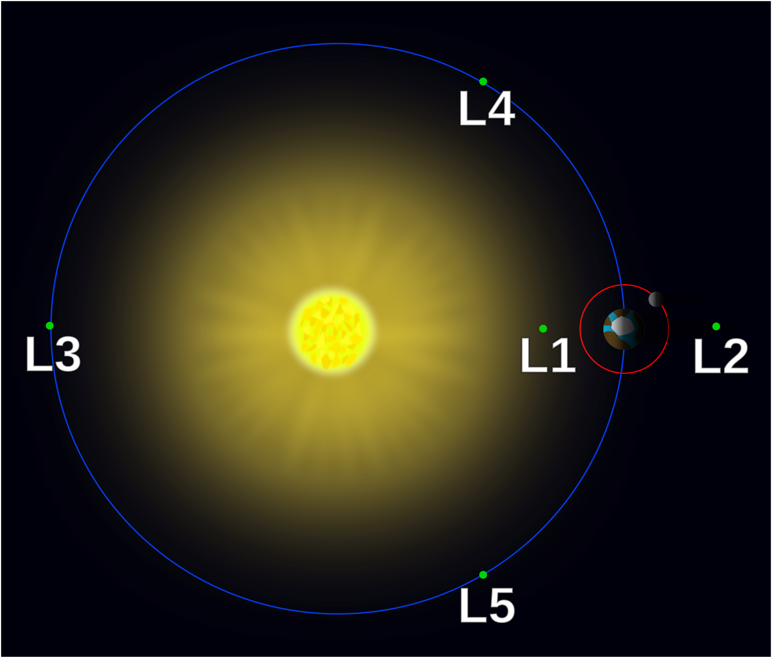 |
|---|
| Figure 5: The five Langrange points for a two-body system like the Sun-Earth system. Created by Xander89 for Wikipedia under the CC BY 3.0 license. |
L4 and L5 are really cool because they show up like the following:
 |
|---|
| Figure 6: Asteroids ‘caught’ at the Jupiter-Sun system’s L4 and L5 points (named Trojans and Greeks respectively :). Source: Wolfram’s YouTube video |
References
- The Wikipedia article on Lagrange Points is a great starting point, as expected.
- Neil J. Cornish’s (1998) article on The Lagrange Points offers a different but useful perspective.
- I created the animations using VPython based on the code introduced in this interesting Dot Physics video.
- Gemini gave useful pointers, in particular for the binomial approximation.