
Preface
You can simulate a lot of things on Earth, but how do you simulate space on Earth?
If you want to send some robots to space, for instance, then how do you test them under the gravitational conditions found on the International Space Station, Moon, or Mars? You obviously cannot just test them on Earth and hope for the best.
This is how I entered this rabbit hole of simulating space on Earth. There are only a handful of options, and parabolic flights hit the sweet spot in many ways, so that’s the one that interested me the most. And it is definitely the coolest.
 |
|---|
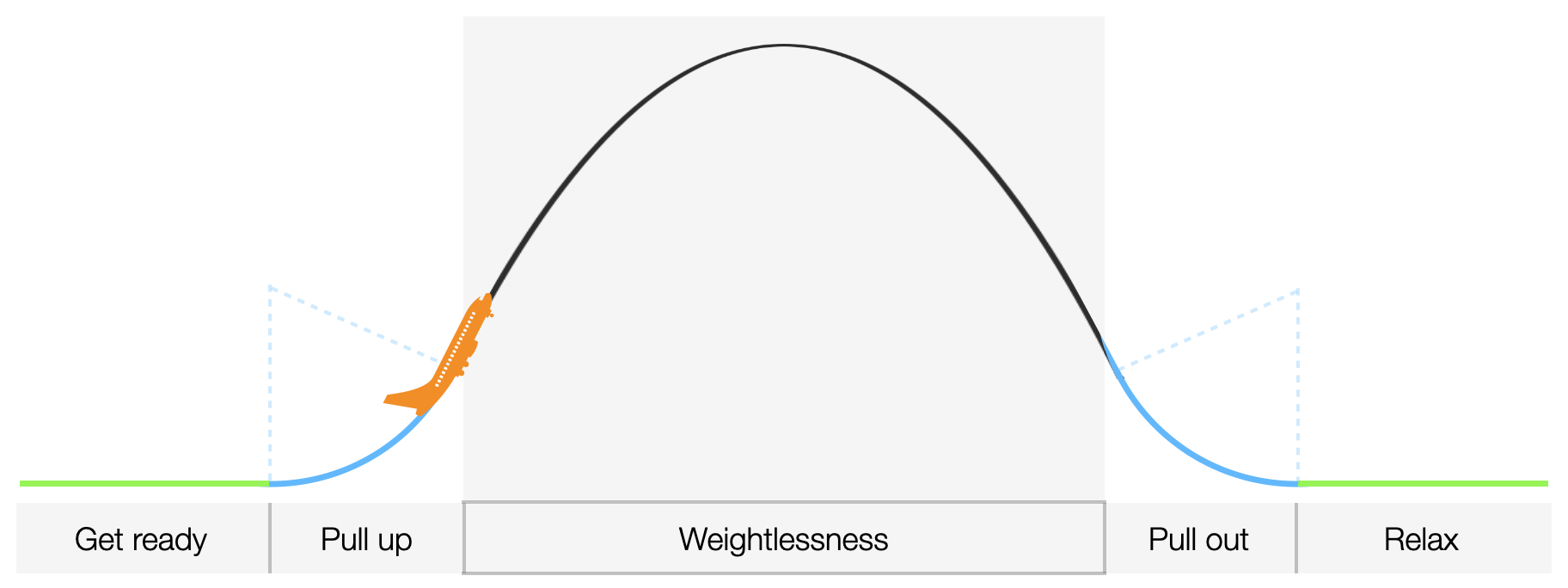
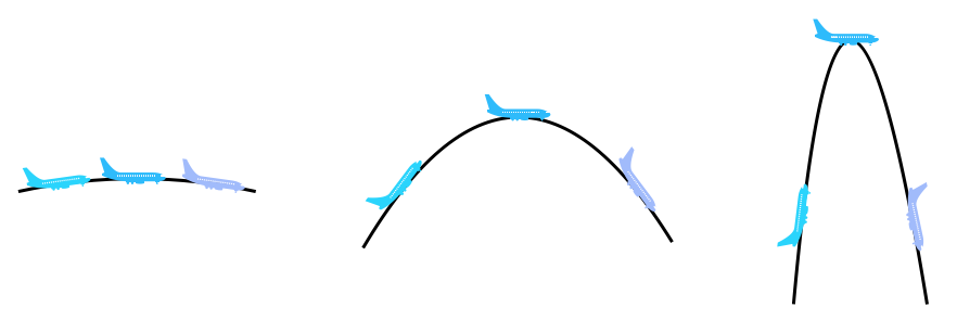
| Figure 1: A typical parabolic-flight pattern. |
So here’s how I understand parabolic flights. Hope you do too.
The outline of this post:
- Deriving that an object thrown with some velocity and angle follows a parabolic path in free-fall (without air resistance)
- What an aircraft has to do to overcome the air resistance and experience free-fall
- Choosing the optimal angle—if any—at which the aircraft should enter the free-fall period
- Understanding how the g-forces acting on the aircraft and its passengers change from g to ~2g to 0g during the parabolic-flight pattern
1. Introduction
In a nutshell, a parabolic flight involves flying an aircraft in a particular repeating pattern such that the passengers feel weightless for about 20 seconds at a time, for about 30 times.
The repeating pattern consists of flying level for a while, then turning up to gain some altitude, then almost turning the engines off for a bit so that the aircraft—and everything inside it—is in free-fall, before the engines are turned up to pull out of the dive and level out the aircraft again. And repeat.
What does this achieve? The middle period when the engines are turned down is similar to throwing a ball towards a friend. The ball has some initial velocity at the instant it leaves your hand, and it is under the effect of gravity till it reaches your friend’s hands. This is called a projectile motion.
 |
|---|
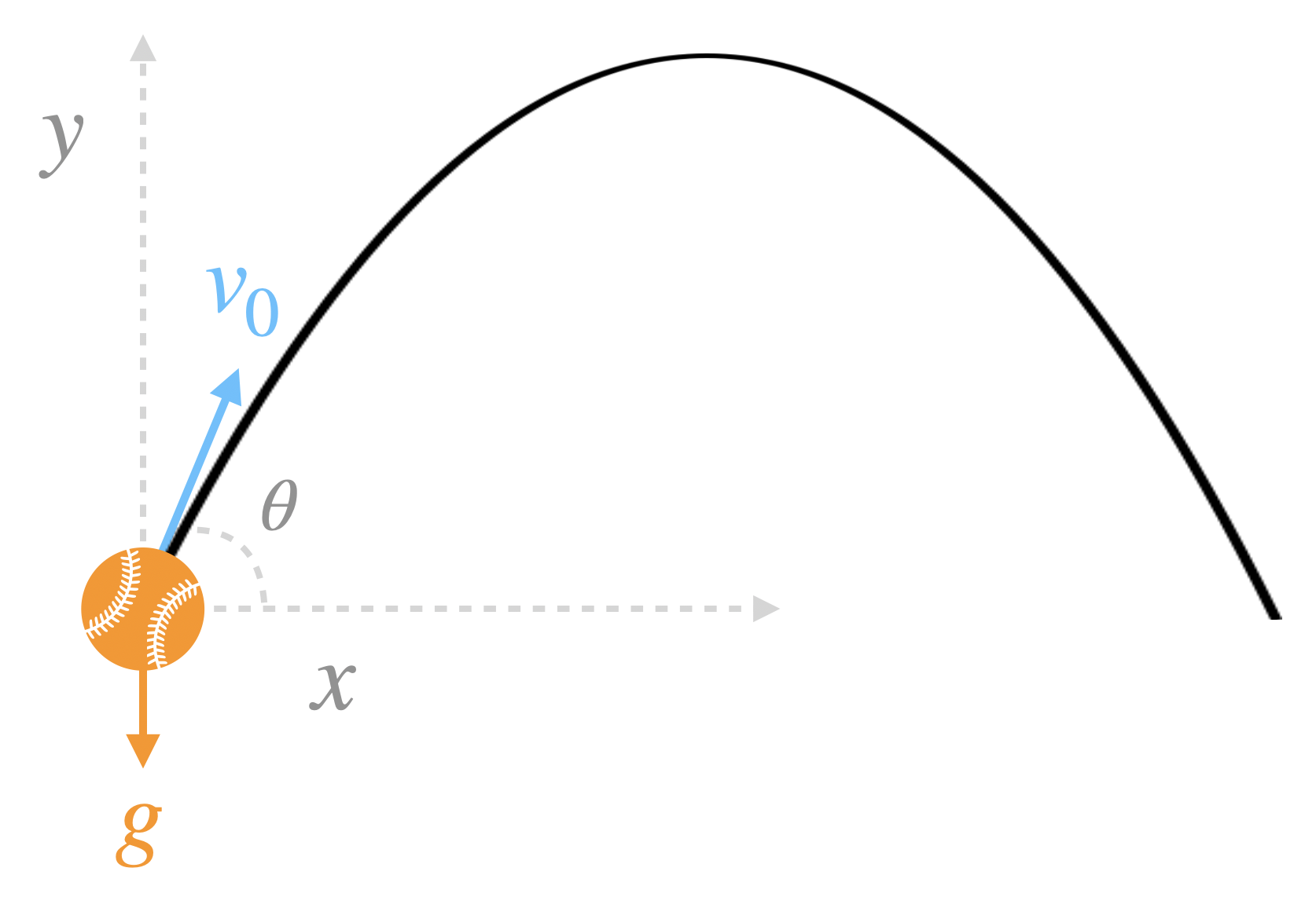
| Figure 2: The path followed by a ball thrown with some initial velocity \(v_0\) at some angle \(\theta\). |
First things first, let’s show that the projection motion follows a parabolic path when there is no air resistance.
\[\begin{align*} \ddot{x}_t &= 0, \\ \ddot{y}_t &= -g. \\ \end{align*}\]Integrating and setting the initial conditions:
\[\begin{align*} \dot{x}_t &= v_0 \cos\theta, \\ \dot{y}_t &= -gt + v_0\sin\theta. \end{align*}\]One more time:
\[\begin{align*} x_t &= v_0 \cos\theta\, t + x_0, \\ y_t &= -\frac{1}{2}gt^2 + v_0\sin\theta\, t + y_0. \end{align*}\]Substituting \(x_t\) in \(y_t\),
\[\begin{align*} y_t = -\frac{1}{2}g \Big(\frac{x_t - x_0}{v_0 \cos\theta}\Big)^2 + v\sin\theta \Big(\frac{x_t - x_0}{v_0 \cos\theta}\Big) + y_0 \end{align*}\]Recall from high-school mathematics that the general equation of a parabola is \(y = ax^2 + bx + c\).
Hence, we have shown that a thrown object solely under the influence of gravity follows a parabolic trajectory.
Great.
If the aircraft was in vacuum and turned its engines off, then it would follow a parabolic trajectory as we showed above.
However, the aircraft is traveling through Earth’s atmosphere and will experience a drag-force opposite to the direction of motion. So if the aircraft’s engines are turned off, then the aircraft would experience a deceleration (causing the passengers to be thrown towards the cabin—much like when a bus brakes/decelerates hard and standing passengers are thrown towards the front).
2. Overcoming air resistance
To counter the deceleration caused by atmospheric drag, the aircraft needs to keep its engines on—just enough to balance the atmospheric drag. If the thrust provided by the engine is greater than the drag, then the passengers will be pushed into their seats; if the thrust is lower than the drag, they will be pushed forward.
Turns out that controlling the thrust requires precise control by the pilots because the atmospheric drag changes continuously due to the changing velocity and height of the aircraft.
 |
|---|
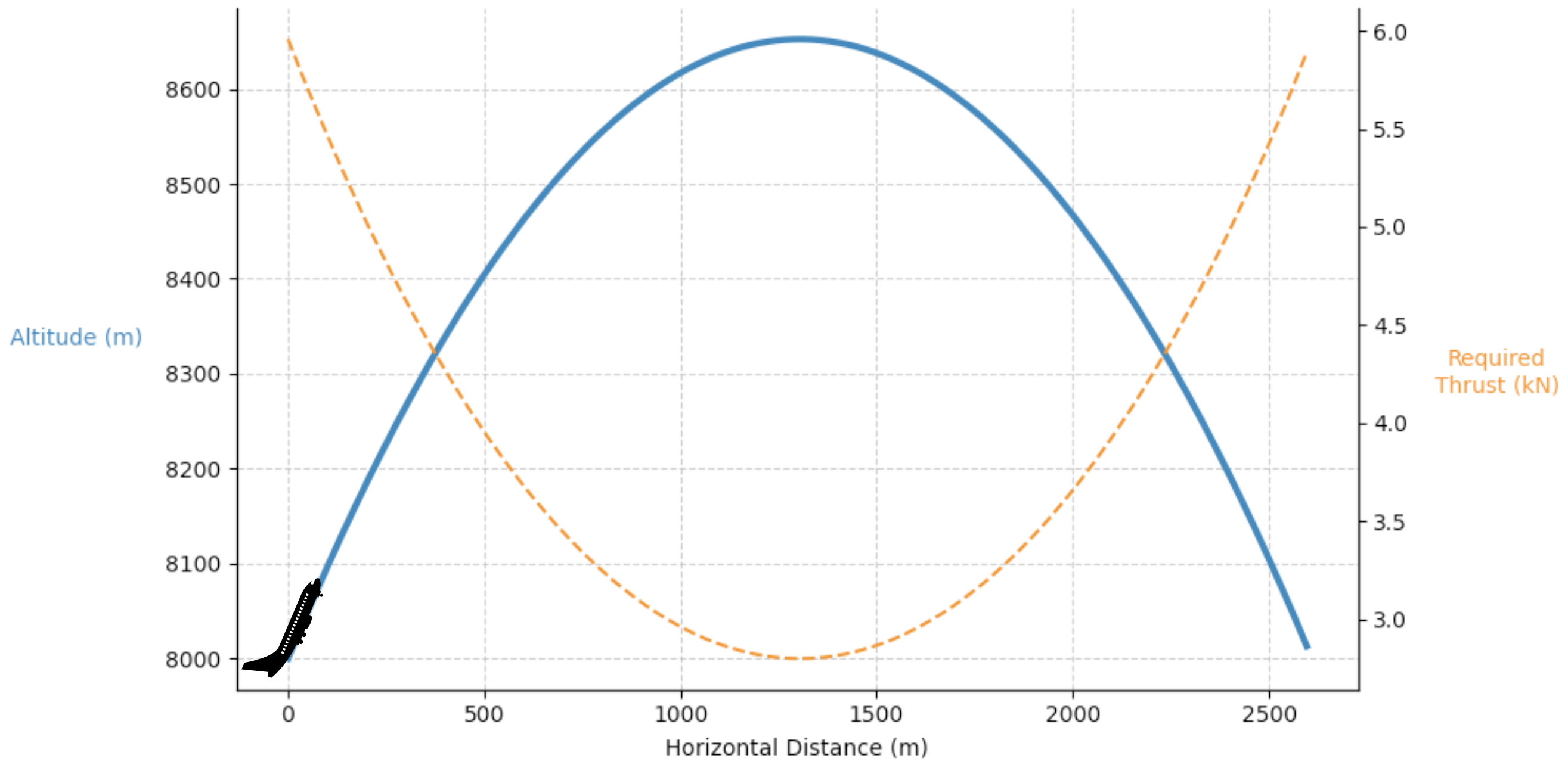
| Figure 3: Thrust required by the airplane engines to negate atmospheric drag. |
I used the following equation for drag: \(\begin{align*} F_d \doteq \frac{1}{2}\rho v^2 c_d A, \end{align*}\) where, \(F_d\) denotes the drag-force, \(\rho\) denotes the density of the fluid in which the object is traveling, \(v\) denotes the velocity of the object w.r.t. the fluid, \(c_d\) is the drag coefficient, and \(A\) denotes the surface area of the object in the direction of motion2.
Note that while the aircraft is in the free-fall phase, its velocity changes—changing the drag. The drag depends on the square of the velocity. And the square of the velocity is linear in the square of time, implying the drag depends on the square of time, or that the drag has a parabolic shape w.r.t. time, just as we see in the above plot.
Here is the complete code to generate the above plot. (And yes, there is a good reason why I chose the Falcon 20 aircraft for reference!)
import jax.numpy as jnp
import matplotlib.pyplot as plt

# Constants
g = 9.81           # m/s^2
m = 10_000         # Mass of an empty Falcon 20 + crew + researchers + equipment (kg; 7500+~2500)
Cd = 0.02          # Drag coefficient
A = 41             # Wing area (m^2; for aircrafts, wing area is considered instead of frontal area)
rho_0 = 1.225      # Air density at sea level (kg/m^3)
H_scale = 10400    # Scale height for density (m)

# Initial conditions for the 20-second parabola
v_0 = 160           # Starting velocity (m/s)
y_0 = 8000          # Initial altitude (m)
theta = jnp.deg2rad(45)  # Entry angle

duration = 23      # simulation duration
dt = 0.05
t = jnp.arange(0, duration, dt)

def simulate_parabola(t, v_0, y_0, theta):
    # velocity components under projectile motion (assuming drag is negated)
    v_x = v_0 * jnp.cos(theta)
    v_y = v_0 * jnp.sin(theta) - g * t
    v_mag = jnp.sqrt(v_x**2 + v_y**2)

    # distance and altitude
    x = v_0 * jnp.cos(theta) * t
    y = y_0 + (v_0 * jnp.sin(theta) * t) - (0.5 * g * t**2)

    # air density: rho(h) = rho_0 * exp(-h / H_scale)
    rho = rho_0 * jnp.exp(-y / H_scale)

    # thrust required is equal and opposite to drag: 0.5 * rho * v^2 * Cd * A
    thrust = 0.5 * rho * (v_mag**2) * Cd * A

    return x, y, thrust

x, y, thrust = simulate_parabola(t, v_0, y_0, theta)

# plotting the results
fig, ax1 = plt.subplots(figsize=(10, 5))

# plot trajectory
ax1.set_xlabel('Horizontal Distance (m)')
ax1.set_ylabel('Altitude (m)', color='tab:blue', rotation=0, labelpad=40)
ax1.plot(x, y, color='tab:blue', linewidth=3)#, label='Flight Path')
ax1.tick_params(axis='y')
ax1.grid(True, linestyle='--', alpha=0.7)
ax1.spines[['top']].set_visible(False)

# plot required thrust
ax2 = ax1.twinx()
ax2.set_ylabel('Required\nThrust (kN)', color='tab:orange', rotation=0, labelpad=40)
ax2.plot(x, thrust / 1000, color='tab:orange', linestyle='--')#, label='Thrust to Negate Drag')
ax2.tick_params(axis='y')
ax2.spines[['top']].set_visible(False)

fig.tight_layout()
plt.show()
3. Choosing the entry angle
What angle should the aircraft be going at when starting the free fall?
45 degrees? That’s the first angle that comes to mind, right? Years of playing cricket reminded me that throwing a ball at roughly 45 degrees maximizes the distance. But maximizing the distance is not the objective here, is it?
What is the objective? Maximizing the amount of time of the weightlessness feeling sounds like a reasonable guess. It would enable performing as many experiments as possible, to get used to being in space, etc.
The duration of weightlessness is easy to compute. Assuming the aircraft thrust negates the atmospheric drag, the duration is simply how long it takes for the vertical upward component of the entry velocity to turn into, say, the equivalent downward component. So, the upward \(v \sin(\theta)\) turns into downward \(-v \sin(\theta)\) under the effect of gravity:
\[\begin{align*} v_{\text{final}} &= v_{\text{initial}} - gt \\ \implies t &= \frac{2v \sin(\theta)}{g}. \end{align*}\]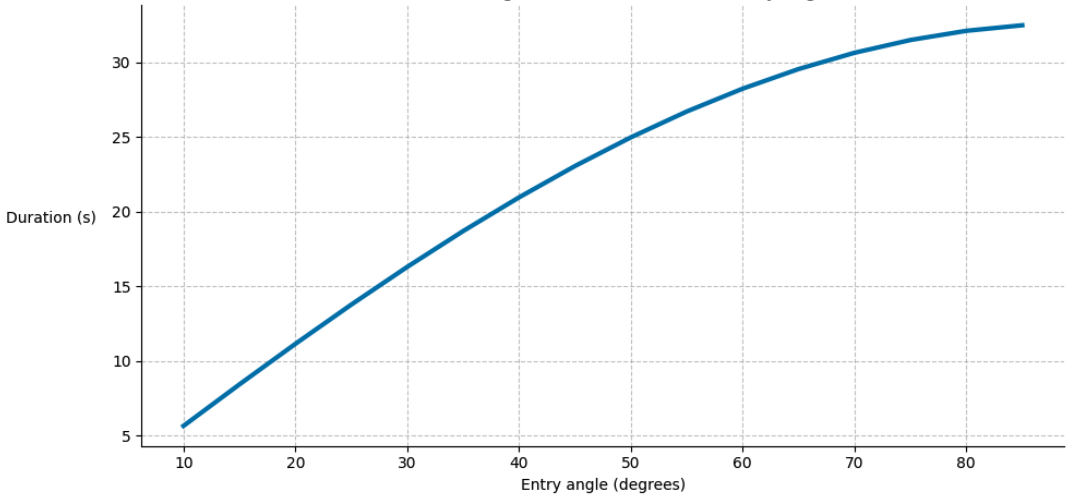 |
|---|
| Figure 4: Duration of weightlessness with different entry angles (for a given entry velocity of 160m/s). |
Clearly, larger the angle, larger the time of flight. So should the aircraft start the weightlessness phase at 90 degrees?
Not really. Consider the amount of movement required by the aircraft in the forward direction (called pitch) at the top of the parabolic arc.
 |
|---|
| Figure 5: The aircraft has to pitch increasingly more at the top of the parabolic arc as the angle of entry increases. |
As the angle of entry increases, the horizontal component of the entry velocity reduces. An aircraft needs to maintain a certain minimum velocity otherwise it risks becoming an uncontrollable metallic tube falling from the sky. In the case of parabolic flights, a certain horizontal velocity is required at the top of the parabola for the pilots to have enough control authority to pitch the aircraft into the dive. This is a little difficult to explain in short and requires reviewing the principles of flight, so you’ll have to take my word for now.
Typically, the entry angle of a parabolic flight is 45—50 degrees3 to balance this tradeoff between increasing duration of weightlessness and decreasing control over the aircraft.
4. 1g to 2g to 0g to 2g to 1g
The next thing to consider is the g-forces acting on the aircraft and its passengers before and after the duration of weightlessness.
 |
|---|
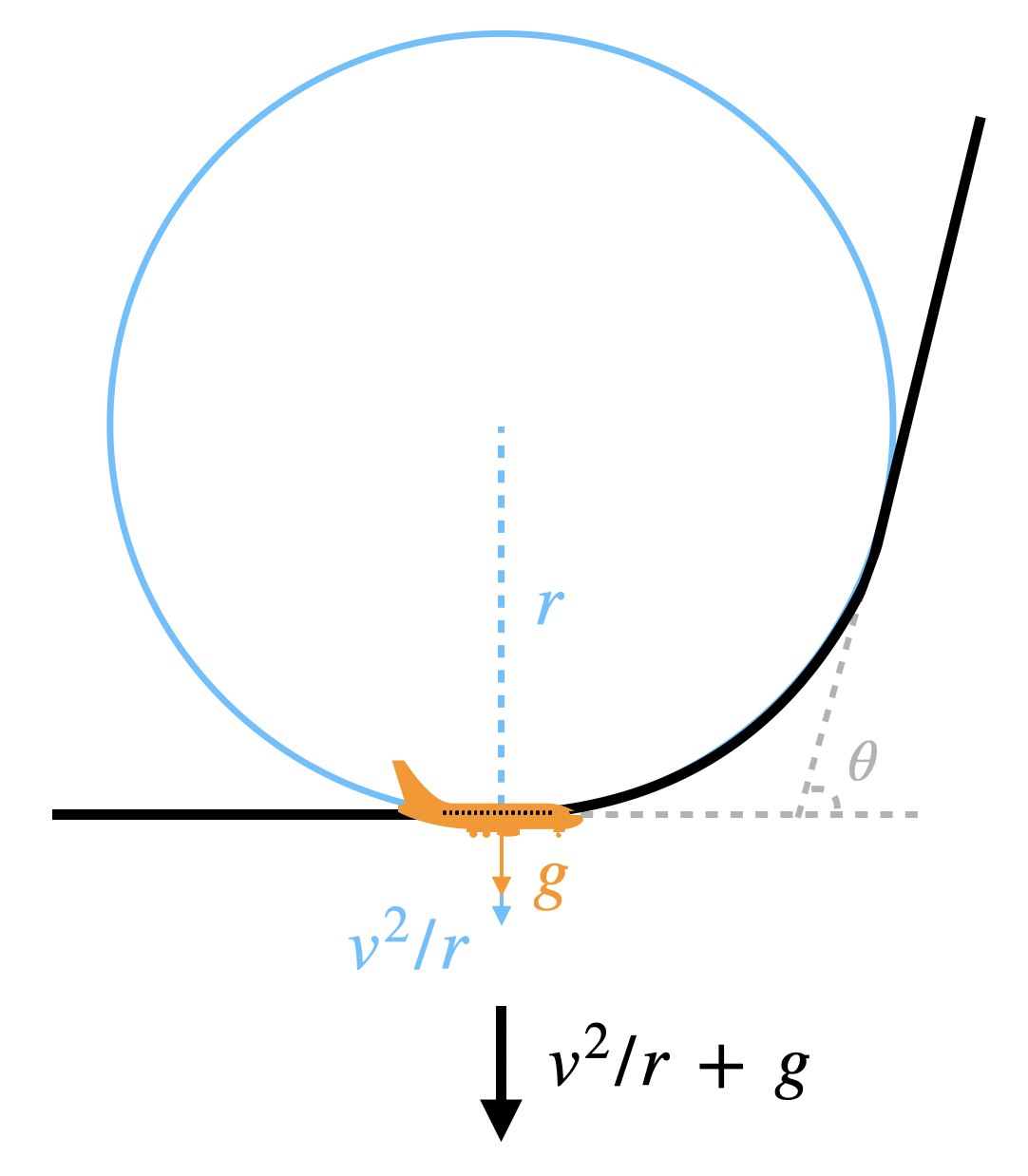
| Figure 6: The net downward force on the aircraft and its passengers is from the acceleration due gravity and the outward centrifugal force from the circular pull-up arc that the aircraft flies to enter the parabolic weightlessness phase. |
The net g-force force at the beginning of a circular pull-up arc is \(g + v^2/r\), where \(r\) is the radius of curvature and \(v\) is the entry velocity.
 |
|---|
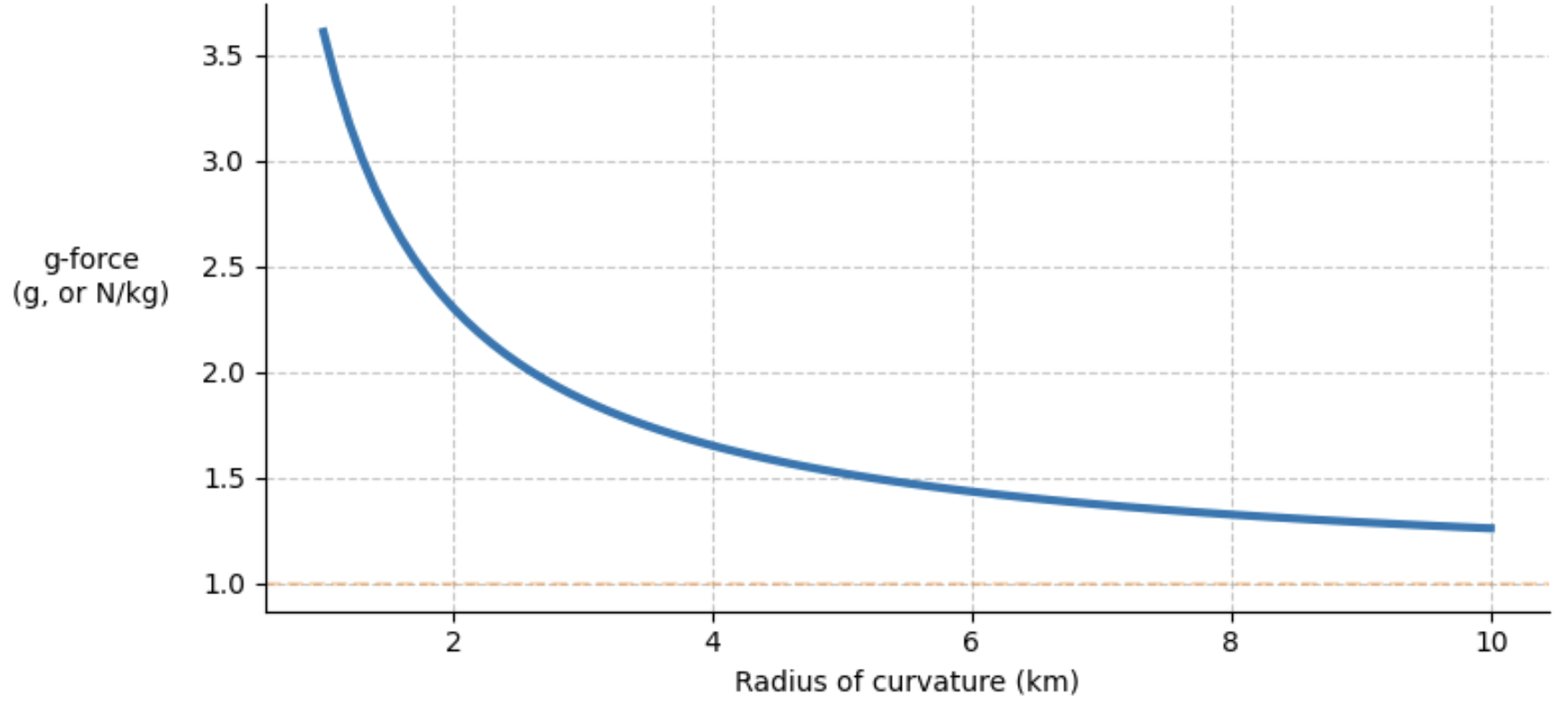
| Figure 7: The net g-force on the aircraft and its passengers for a given entry velocity (160 m/s). |
According to Wikipedia, modern commercial aircrafts are designed to withstand g-forces up to +2.5g.
Aircrafts for parabolic flights are retrofitted to withstand more g-forces that a commercial aircraft, but the next consideration is also how much g-forces the human passengers can handle. Fighter pilots can withstand up to 9g for a few seconds; F1 drivers need to handle up to 5g on some circuits; regular folks like you and me may not be comfortable beyond 3g (watch Tom Scott pass out at 3.6g in <10s!).
So why not have a large radius of curvature (like 10km) so that the net g-force is close to \(1g\), something we are evolved for?
Simple answer: to save fuel. Beyond the obvious benefit to the environment, parabolic flights are not cheap (for instance, Novespace charges ~7500 Euros (~12k CAD) for ~10mins of total weightlessness!). More comfort means a lot more fuel and money.
The sweet spot is considered to be about 1.8g. This translates to a radius of curvature ~3km.
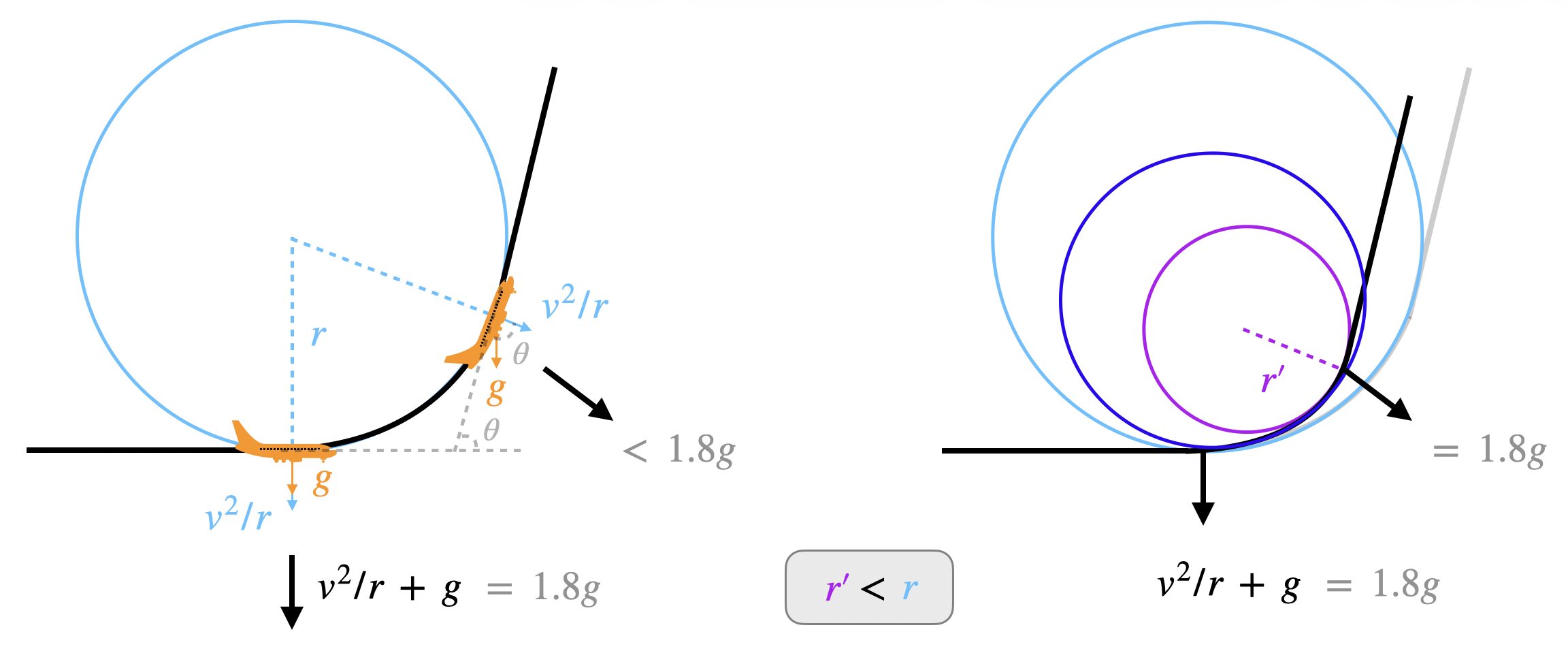
An astute reader may note that the centrifugal force will only completely add with the gravitational force at the bottom of the arc. The total g-force decreases from the starting point to the end of the arc. We know that this makes the ride more comfortable, but for higher fuel efficiency, it makes sense to decrease the radius of curvature and reach the angle of approach faster. The pilots can maintain a g-force of 1.8g on the passengers and the aircraft by making the radius of curvature tighter and tighter from the starting of the arc.
 |
|---|
| Figure 8: To maintain a roughly constant g-force on the aircraft and its passengers, pilots skillfully follow a decreasing radius of curvature. |
Epilogue
So that’s the science and maths behind parabolic flights to simulate microgravity on Earth. I really wish I can try some experiments on a parabolic flight one day.
I want to leave you with one last question. Now that you know how to simulate weightlessness (that is, 0g), how would you modify the flight plan/path to simulate other gravities, such as 0.17g Lunar gravity or 0.38g Martian gravity? Let me know :)
As always, stay curious!
References
- General references: Wikipedia: Reduced-gravity aircraft, Aeroreport: A brief guide: Parabolic flights, CSA: Parabolic Flights
- For estimating the drag: A page on NASA’s website
- For the angle of entry: 1, 2, 3, 4, 5
I got a bunch of preliminary information from Gemini, after which I went down a bunch of rabbit holes to put together this post. I created all the plots using JAX/matplotlib and created all the visualizations using Keynote.